UPGMA

UPGMA （unweighted pair group method with arithmetic mean）是一種相對簡單的層次聚類方法。這個方法存在另一種變體 WPGMA。這個方法的創始人被認為是Sokal和Michener 。 ^[1]

演算方法

UPGMA 演法構建出一棵有根樹（樹狀圖）表現相似矩陣或相異矩陣中的特徵與結構。在算法裡的每一步，距離最近的兩個集群（子樹）將被組合成一個更高級別的集群。任意兩個集群${\displaystyle {\mathcal {A}}}$和${\displaystyle {\mathcal {B}}}$ 之間的距離，是由所有${\displaystyle {\mathcal {A}}}$裡的${\displaystyle x}$元素和所有${\displaystyle {\mathcal {B}}}$裡的${\displaystyle y}$元素的距離${\displaystyle d(x,y)}$的平均值，即每個集群的元素之間的平均距離，其中 ${\displaystyle {|{\mathcal {A}}|}}$和${\displaystyle {|{\mathcal {B}}|}}$是該兩個集群的基數（集合大小）：

${\displaystyle d_{{\mathcal {A}},{\mathcal {B}}}={1 \over {|{\mathcal {A}}|\cdot |{\mathcal {B}}|}}\sum _{x\in {\mathcal {A}}}\sum _{y\in {\mathcal {B}}}d(x,y)}$

換句話說，在每一次組合成新集群的步驟中，可以由${\displaystyle d_{{\mathcal {A}},X}}$和${\displaystyle d_{{\mathcal {B}},X}}$的加權平均給出集群${\displaystyle {\mathcal {A}}\cup {\mathcal {B}}}$和一個新集群${\displaystyle X}$之間的距離：

${\displaystyle d_{({\mathcal {A}}\cup {\mathcal {B}}),X}={\frac {|{\mathcal {A}}|\cdot d_{{\mathcal {A}},X}+|{\mathcal {B}}|\cdot d_{{\mathcal {B}},X}}{|{\mathcal {A}}|+|{\mathcal {B}}|}}}$

UPGMA 演算法生成的有根樹狀圖是一個超度量樹，該樹需要套用等速率的假設，也就是說根到每個分支尖端的距離皆相等。當尖端是同時採樣的分子數據（即DNA 、 RNA和蛋白質）時，超度量假設就等同於分子鐘假設。

示例

這個示例是基於JC69基因距離矩陣，該矩陣是根據五種細菌的5S 核糖體 RNA序列計算出來的，五種細菌如下所列^{[2] [3]}：

枯草桿菌 Bacillus subtilis( ${\displaystyle a}$ )

嗜热脂肪芽孢杆菌 <i>Bacillus stearothermophilus</i>( ${\displaystyle b}$ )

魏斯氏菌 Lactobacillus viridescens( ${\displaystyle c}$ )

無原枯草桿菌 Acholeplasma modicum( ${\displaystyle d}$ )

藤黄微球菌 <i>Micrococcus luteus</i>( ${\displaystyle e}$ )

第一步

• 首次集群

假設有五個物件${\displaystyle (a,b,c,d,e)}$和他們之間的相異矩陣${\displaystyle D_{1}}$：

	a	b	c	d	e
a	0	17	21	31	23
b	17	0	30	34	21
c	21	30	0	28	39
d	31	34	28	0	43
e	23	21	39	43	0

在這裡，${\displaystyle D_{1}(a,b)=17}$是最小值，所以將${\displaystyle a}$和${\displaystyle b}$集群。

• 第一分支長度估計

令${\displaystyle u}$表示現在${\displaystyle a}$ 和 ${\displaystyle b}$ 的祖先。為了讓${\displaystyle a}$ 和 ${\displaystyle b}$ 與 ${\displaystyle u}$等距，假設${\displaystyle \delta (a,u)=\delta (b,u)=D_{1}(a,b)/2}$，這對應到了超度量的假設。在這個範例中：${\displaystyle \delta (a,u)=\delta (b,u)=17/2=8.5}$

• 第一次相異矩陣更新

然後將${\displaystyle D_{1}}$更新成一個新的距離矩陣${\displaystyle D_{2}}$（計算在下方），由於${\displaystyle a}$和${\displaystyle b}$的集群，該矩陣的尺寸減少了一行一列。（${\displaystyle D_{2}}$中粗體表示的值是由加權平均計算出的新距離）

${\displaystyle D_{2}((a,b),c)=(D_{1}(a,c)\times 1+D_{1}(b,c)\times 1)/(1+1)=(21+30)/2=25.5}$

${\displaystyle D_{2}((a,b),d)=(D_{1}(a,d)+D_{1}(b,d))/2=(31+34)/2=32.5}$

${\displaystyle D_{2}((a,b),e)=(D_{1}(a,e)+D_{1}(b,e))/2=(23+21)/2=22}$

${\displaystyle D_{2}}$中的斜體值不受矩陣更新影響，因為他們與第一個集群中的元素完全美有關連。

第二步

• 第二次集群

現在重複前面的三個步驟，並從新的相異矩陣${\displaystyle D_{2}}$開始

	(a,b)	ｃ	d	ｅ
(a,b)	0	25.5	32.5	22
ｃ	25.5	0	28	39
d	32.5	28	0	43
ｅ	22	39	43	0

在這個矩陣中， ${\displaystyle D_{2}((a,b),e)=22}$是${\displaystyle D_{2}}$中的最小值，所以將${\displaystyle (a,b)}$和元素${\displaystyle e}$集成新群。

• 第二次分支長度估計

令${\displaystyle v}$表示節點${\displaystyle (a,b)}$和${\displaystyle e}$的祖先。由超度量假設可以得到${\displaystyle a,b,e}$三頂點到${\displaystyle v}$的距離相等，即：${\displaystyle \delta (a,v)=\delta (b,v)=\delta (e,v)=22/2=11}$，從而可以計算出${\displaystyle u}$到${\displaystyle v}$的距離${\displaystyle \delta (u,v)=\delta (e,v)-\delta (a,u)=\delta (e,v)-\delta (b,u)=11-8.5=2.5}$

• 第二次距離矩陣更新

然後將${\displaystyle D_{2}}$更新成新的距離矩陣${\displaystyle D_{3}}$，數值計算如下：

${\displaystyle D_{3}(((a,b),e),c)=(D_{2}((a,b),c)\times 2+D_{2}(e,c)\times 1)/(2+1)=(25.5\times 2+39\times 1)/3=30}$

${\displaystyle D_{3}(((a,b),e),d)=(D_{2}((a,b),d)\times 2+D_{2}(e,d)\times 1)/(2+1)=(32.5\times 2+43\times 1)/3=36}$

第三、四步

重複上述動作可以得到${\displaystyle D_{3}}$是

	((a,b),e)	c	d
((a,b),e)	0	30	36
c	30	0	28
d	36	28	0

${\displaystyle D_{4}}$是：

	((a,b),e)	（c,d）
((a,b),e)	0	33
（c,d）	33	0

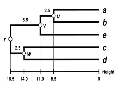
UPGMA樹狀圖

這裡顯示了完成的樹狀圖。^[4]它是超度量的，所有尖端（ ${\displaystyle a}$到${\displaystyle e}$ ) 與${\displaystyle r}$等距離 :

${\displaystyle \delta (a,r)=\delta (b,r)=\delta (e,r)=\delta (c,r)=\delta (d,r)=16.5}$

這個樹狀圖的根是它最深的節點${\displaystyle r}$ 。

時間複雜度

構建 UPGMA 樹的算法有${\displaystyle O(n^{3})}$時間複雜度。使用一個堆維護兩個即群之間的距離可以使時間達到${\displaystyle O(n^{2}\log n)}$ . 另外Fionn Murtagh 提出了一個${\displaystyle O(n^{2})}$時空複雜度的算法。 ^[5]

See also

• 鄰接法
• 集群分析
• 单链接聚类
• 完全连锁聚类
• 層次即群
• DNA进化模型
• 分子鐘

外部連結

• UPGMA聚类算法在Ruby中的实现（AI4R） （页面存档备份，存于互联网档案馆）
• 使用相似矩阵计算 UPGMA 的示例 （页面存档备份，存于互联网档案馆）
• 使用距离矩阵计算 UPGMA 的示例 （页面存档备份，存于互联网档案馆）