Trigonometri Garis besar Sejarah Kegunaan Fungsi (invers) Trigonometri rampat Rujukan Aturan dan teorema Sinus Kosinus Tangen Kotangen Kalkulus Substitusi trigonometri Integral (fungsi invers) Turunan
Trigonometri merupakan salah satu cabang matematika yang mempelajari sudut dalam segitiga siku-siku (yang dijelaskan secara geometri). Identitas trigonometri merupakan salah satu fungsi trigonometri dimana rumus tersebut memiliki hasil yang sama bila diuji suatu nilai variabel. Identitas berikut ini sangatlah penting dan berguna dalam komputasi yang elusif.
Daftar ini menjelaskan dasar-dasar fungsi, invers fungsi, beserta nilai sudut istimewa pada fungsi trigonometri. Dan juga mengenai jumlah dan perkalian sudut. Mengenai daftar identitas fungsi invers juga dimasukkan ke dalam halaman ini. Terdapat bukti-bukti mengenai rumus-rumus di bawah. Meski begitu, halaman ini hanya menjelaskan bukti singkat pada rumus dan adapula yang tidak. Untuk melihat bukti, lihat Bukti identitas trigonometri. Berikut adalah daftar identitas trigonometri .
Fungsi dasar trigonometri Segitiga siku-siku A B C {\displaystyle ABC} A C = b {\displaystyle AC=b} B C = a {\displaystyle BC=a} A B = c {\displaystyle AB=c} Salah satu fungsi trigonometri paling umum, semenjak kita duduk di bangku sekolah menengah atas adalah fungsi trigonometri seperti sinus, kosinus, tangen, sekan, kosekan, dan kotangen. Secara geometri, keenam fungsi trigonometri tersebut dapat didefinisikan melalui sudut pada segitiga. Misalkan A B C {\displaystyle ABC} a {\displaystyle a} b {\displaystyle b} c {\displaystyle c} A {\displaystyle A}
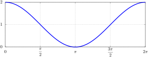
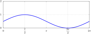
sin A = a c {\displaystyle \sin A={\frac {a}{c}}} cos A = b c {\displaystyle \cos A={\frac {b}{c}}} tan A = a b = sin A cos A {\displaystyle \tan A={\frac {a}{b}}={\frac {\sin A}{\cos A}}} cot A = 1 tan A = cos A sin A = b a {\displaystyle \cot A={\frac {1}{\tan A}}={\frac {\cos A}{\sin A}}={\frac {b}{a}}} sec A = 1 cos A = c b {\displaystyle \sec A={\frac {1}{\cos A}}={\frac {c}{b}}} csc A = 1 sin A = c a {\displaystyle \csc A={\frac {1}{\sin A}}={\frac {c}{a}}} Keenam fungsi trigonometri di atas memiliki grafik, dengan ranah dan kisaran pada setiap dari mereka adalah berbeda, terutama periodenya. Berikut adalah daftar fungsi trigonometri yang ditabelkan, dengan periode, ranah, kisaran, beserta visualisasi grafik fungsi.
Fungsi Periode Ranah Kisaran Grafik sinus 2 π {\displaystyle 2\pi } ( − ∞ , ∞ ) {\displaystyle (-\infty ,\infty )} [ − 1 , 1 ] {\displaystyle [-1,1]} kosinus 2 π {\displaystyle 2\pi } ( − ∞ , ∞ ) {\displaystyle (-\infty ,\infty )} [ − 1 , 1 ] {\displaystyle [-1,1]} tangen π {\displaystyle \pi } x ≠ n π {\displaystyle x\neq n\pi } ( − ∞ , ∞ ) {\displaystyle (-\infty ,\infty )} sekan 2 π {\displaystyle 2\pi } x ≠ π 2 + n π {\displaystyle x\neq {\frac {\pi }{2}}+n\pi } ( − ∞ , − 1 ] ∪ [ 1 , ∞ ) {\displaystyle (-\infty ,-1]\cup [1,\infty )} kosekan 2 π {\displaystyle 2\pi } x ≠ π 2 + n π {\displaystyle x\neq {\frac {\pi }{2}}+n\pi } ( − ∞ , − 1 ] ∪ [ 1 , ∞ ) {\displaystyle (-\infty ,-1]\cup [1,\infty )} kotangen π {\displaystyle \pi } x ≠ n π {\displaystyle x\neq n\pi } ( − ∞ , ∞ ) {\displaystyle (-\infty ,\infty )}
Nilai sudut istimewa Berikut adalah nilai sudut istimewa pada keenam fungsi trigonometri:
Sinus Kosinus Tangen Kotangen Sekan Kosekan 0° 0 {\displaystyle 0} 1 {\displaystyle 1} 0 {\displaystyle 0} ∞ {\displaystyle \infty } 1 {\displaystyle 1} ∞ {\displaystyle \infty } 8° 2 10 {\displaystyle {\frac {\sqrt {2}}{10}}} 7 2 10 {\displaystyle {\frac {7{\sqrt {2}}}{10}}} 1 7 {\displaystyle {\frac {1}{7}}} 7 {\displaystyle 7} 5 2 7 {\displaystyle {\frac {5{\sqrt {2}}}{7}}} 5 2 {\displaystyle 5{\sqrt {2}}} 15° 6 − 2 4 {\displaystyle {\frac {{\sqrt {6}}-{\sqrt {2}}}{4}}} 6 + 2 4 {\displaystyle {\frac {{\sqrt {6}}+{\sqrt {2}}}{4}}} 2 − 3 {\displaystyle 2-{\sqrt {3}}} 2 + 3 {\displaystyle 2+{\sqrt {3}}} 6 − 2 {\displaystyle {\sqrt {6}}-{\sqrt {2}}} 6 + 2 {\displaystyle {\sqrt {6}}+{\sqrt {2}}} 16° 7 25 {\displaystyle {\frac {7}{25}}} 24 25 {\displaystyle {\frac {24}{25}}} 7 24 {\displaystyle {\frac {7}{24}}} 24 7 {\displaystyle {\frac {24}{7}}} 25 24 {\displaystyle {\frac {25}{24}}} 25 7 {\displaystyle {\frac {25}{7}}} 18° − 1 + 5 4 {\displaystyle {\frac {-1+{\sqrt {5}}}{4}}} 10 + 2 5 4 {\displaystyle {\frac {\sqrt {10+2{\sqrt {5}}}}{4}}} ( − 5 + 3 5 ) 10 + 2 5 20 {\displaystyle {\frac {(-5+3{\sqrt {5}}){\sqrt {10+2{\sqrt {5}}}}}{20}}} ( 1 + 5 ) 10 + 2 5 4 {\displaystyle {\frac {(1+{\sqrt {5}}){\sqrt {10+2{\sqrt {5}}}}}{4}}} ( 5 − 5 ) 10 + 2 5 10 {\displaystyle {\frac {(5-{\sqrt {5}}){\sqrt {10+2{\sqrt {5}}}}}{10}}} 1 + 5 {\displaystyle 1+{\sqrt {5}}} 30° 1 2 {\displaystyle {\frac {1}{2}}} 3 2 {\displaystyle {\frac {\sqrt {3}}{2}}} 3 3 {\displaystyle {\frac {\sqrt {3}}{3}}} 3 {\displaystyle {\sqrt {3}}} 2 3 3 {\displaystyle {\frac {2{\sqrt {3}}}{3}}} 2 {\displaystyle 2} 36° 10 − 2 5 4 {\displaystyle {\frac {\sqrt {10-2{\sqrt {5}}}}{4}}} 1 + 5 4 {\displaystyle {\frac {1+{\sqrt {5}}}{4}}} ( − 1 + 5 ) 10 − 2 5 4 {\displaystyle {\frac {(-1+{\sqrt {5}}){\sqrt {10-2{\sqrt {5}}}}}{4}}} ( 5 + 3 5 ) 10 − 2 5 20 {\displaystyle {\frac {(5+3{\sqrt {5}}){\sqrt {10-2{\sqrt {5}}}}}{20}}} − 1 + 5 {\displaystyle -1+{\sqrt {5}}} ( 5 + 5 ) 10 − 2 5 10 {\displaystyle {\frac {(5+{\sqrt {5}}){\sqrt {10-2{\sqrt {5}}}}}{10}}} 37° 3 5 {\displaystyle {\frac {3}{5}}} 4 5 {\displaystyle {\frac {4}{5}}} 3 4 {\displaystyle {\frac {3}{4}}} 4 3 {\displaystyle {\frac {4}{3}}} 5 4 {\displaystyle {\frac {5}{4}}} 5 3 {\displaystyle {\frac {5}{3}}} 45° 2 2 {\displaystyle {\frac {\sqrt {2}}{2}}} 2 2 {\displaystyle {\frac {\sqrt {2}}{2}}} 1 {\displaystyle 1} 1 {\displaystyle 1} 2 {\displaystyle {\sqrt {2}}} 2 {\displaystyle {\sqrt {2}}} 53° 4 5 {\displaystyle {\frac {4}{5}}} 3 5 {\displaystyle {\frac {3}{5}}} 4 3 {\displaystyle {\frac {4}{3}}} 3 4 {\displaystyle {\frac {3}{4}}} 5 3 {\displaystyle {\frac {5}{3}}} 5 4 {\displaystyle {\frac {5}{4}}} 54° 1 + 5 4 {\displaystyle {\frac {1+{\sqrt {5}}}{4}}} 10 − 2 5 4 {\displaystyle {\frac {\sqrt {10-2{\sqrt {5}}}}{4}}} ( 5 + 3 5 ) 10 − 2 5 20 {\displaystyle {\frac {(5+3{\sqrt {5}}){\sqrt {10-2{\sqrt {5}}}}}{20}}} ( − 1 + 5 ) 10 − 2 5 4 {\displaystyle {\frac {(-1+{\sqrt {5}}){\sqrt {10-2{\sqrt {5}}}}}{4}}} ( 5 + 5 ) 10 − 2 5 10 {\displaystyle {\frac {(5+{\sqrt {5}}){\sqrt {10-2{\sqrt {5}}}}}{10}}} − 1 + 5 {\displaystyle -1+{\sqrt {5}}} 60° 3 2 {\displaystyle {\frac {\sqrt {3}}{2}}} 1 2 {\displaystyle {\frac {1}{2}}} 3 {\displaystyle {\sqrt {3}}} 3 3 {\displaystyle {\frac {\sqrt {3}}{3}}} 2 {\displaystyle 2} 2 3 3 {\displaystyle {\frac {2{\sqrt {3}}}{3}}} 72° 10 + 2 5 4 {\displaystyle {\frac {\sqrt {10+2{\sqrt {5}}}}{4}}} − 1 + 5 4 {\displaystyle {\frac {-1+{\sqrt {5}}}{4}}} ( 1 + 5 ) 10 + 2 5 4 {\displaystyle {\frac {(1+{\sqrt {5}}){\sqrt {10+2{\sqrt {5}}}}}{4}}} ( − 5 + 3 5 ) 10 + 2 5 20 {\displaystyle {\frac {(-5+3{\sqrt {5}}){\sqrt {10+2{\sqrt {5}}}}}{20}}} 1 + 5 {\displaystyle 1+{\sqrt {5}}} ( 5 − 5 ) 10 + 2 5 10 {\displaystyle {\frac {(5-{\sqrt {5}}){\sqrt {10+2{\sqrt {5}}}}}{10}}} 74° 24 25 {\displaystyle {\frac {24}{25}}} 7 25 {\displaystyle {\frac {7}{25}}} 24 7 {\displaystyle {\frac {24}{7}}} 7 24 {\displaystyle {\frac {7}{24}}} 25 7 {\displaystyle {\frac {25}{7}}} 25 24 {\displaystyle {\frac {25}{24}}} 75° 6 + 2 4 {\displaystyle {\frac {{\sqrt {6}}+{\sqrt {2}}}{4}}} 6 − 2 4 {\displaystyle {\frac {{\sqrt {6}}-{\sqrt {2}}}{4}}} 2 + 3 {\displaystyle 2+{\sqrt {3}}} 2 − 3 {\displaystyle 2-{\sqrt {3}}} 6 + 2 {\displaystyle {\sqrt {6}}+{\sqrt {2}}} 6 − 2 {\displaystyle {\sqrt {6}}-{\sqrt {2}}} 82° 7 2 10 {\displaystyle {\frac {7{\sqrt {2}}}{10}}} 2 10 {\displaystyle {\frac {\sqrt {2}}{10}}} 7 {\displaystyle 7} 1 7 {\displaystyle {\frac {1}{7}}} 5 2 {\displaystyle 5{\sqrt {2}}} 5 2 7 {\displaystyle {\frac {5{\sqrt {2}}}{7}}} 90° 1 {\displaystyle 1} 0 {\displaystyle 0} ∞ {\displaystyle \infty } 0 {\displaystyle 0} ∞ {\displaystyle \infty } 1 {\displaystyle 1}
Fungsi invers trigonometri Fungsi invers trigonometri merupakan fungsi yang merupakan kebalikan dari fungsi dasar trigonometri. Lazimnya, fungsi invers trigonometri biasanya dinotasikan dengan prefiks arc -.[1] − 1 {\displaystyle ^{-1}} [nb 1]
Berikut adalah fungsi invers trigonometri, dengan ranah dan kisarannya, antara lain:
Nama fungsi Simbol Ranah Citra/Kisaran Fungsi Ranah Citra sinus sin {\displaystyle \sin } : {\displaystyle :} R {\displaystyle \mathbb {R} } → {\displaystyle \to } [ − 1 , 1 ] {\displaystyle [-1,1]} arcsin {\displaystyle \arcsin } : {\displaystyle :} [ − 1 , 1 ] {\displaystyle [-1,1]} → {\displaystyle \to } [ − π 2 , π 2 ] {\displaystyle \left[-{\tfrac {\pi }{2}},{\tfrac {\pi }{2}}\right]} kosinus cos {\displaystyle \cos } : {\displaystyle :} R {\displaystyle \mathbb {R} } → {\displaystyle \to } [ − 1 , 1 ] {\displaystyle [-1,1]} arccos {\displaystyle \arccos } : {\displaystyle :} [ − 1 , 1 ] {\displaystyle [-1,1]} → {\displaystyle \to } [ 0 , π ] {\displaystyle [0,\pi ]} tangen tan {\displaystyle \tan } : {\displaystyle :} π Z + ( − π 2 , π 2 ) {\displaystyle \pi \mathbb {Z} +\left(-{\tfrac {\pi }{2}},{\tfrac {\pi }{2}}\right)} → {\displaystyle \to } R {\displaystyle \mathbb {R} } arctan {\displaystyle \arctan } : {\displaystyle :} R {\displaystyle \mathbb {R} } → {\displaystyle \to } ( − π 2 , π 2 ) {\displaystyle \left(-{\tfrac {\pi }{2}},{\tfrac {\pi }{2}}\right)} kotangen cot {\displaystyle \cot } : {\displaystyle :} π Z + ( 0 , π ) {\displaystyle \pi \mathbb {Z} +(0,\pi )} → {\displaystyle \to } R {\displaystyle \mathbb {R} } arccot {\displaystyle \operatorname {arccot} } : {\displaystyle :} R {\displaystyle \mathbb {R} } → {\displaystyle \to } ( 0 , π ) {\displaystyle (0,\pi )} sekan sec {\displaystyle \sec } : {\displaystyle :} π Z + ( − π 2 , π 2 ) {\displaystyle \pi \mathbb {Z} +\left(-{\tfrac {\pi }{2}},{\tfrac {\pi }{2}}\right)} → {\displaystyle \to } R ∖ ( − 1 , 1 ) = ( − ∞ , − 1 ] ∪ [ 1 , ∞ ) {\displaystyle \mathbb {R} \setminus (-1,1)=(-\infty ,-1]\cup [1,\infty )} arcsec {\displaystyle \operatorname {arcsec} } : {\displaystyle :} R ∖ ( − 1 , 1 ) {\displaystyle \mathbb {R} \setminus (-1,1)} → {\displaystyle \to } [ 0 , π ] ∖ { π 2 } {\displaystyle [\,0,\;\pi \,]\;\;\;\setminus \left\{{\tfrac {\pi }{2}}\right\}} kosekan csc {\displaystyle \csc } : {\displaystyle :} π Z + ( 0 , π ) {\displaystyle \pi \mathbb {Z} +(0,\pi )} → {\displaystyle \to } R ∖ ( − 1 , 1 ) {\displaystyle \mathbb {R} \setminus (-1,1)} arccsc {\displaystyle \operatorname {arccsc} } : {\displaystyle :} R ∖ ( − 1 , 1 ) {\displaystyle \mathbb {R} \setminus (-1,1)} → {\displaystyle \to } [ − π 2 , π 2 ] ∖ { 0 } {\displaystyle \left[-{\tfrac {\pi }{2}},{\tfrac {\pi }{2}}\right]\setminus \{0\}}
Komposisi fungsi trigonometri dengan invers fungsinya sendiri akan sama dengan menuliskan suatu variabel. Dengan kata lain (tinjau f {\displaystyle f}
f ( f − 1 ( x ) ) = x {\displaystyle f(f^{-1}(x))=x} f − 1 ( f ( x ) ) = x {\displaystyle f^{-1}(f(x))=x} Hal yang serupa untuk fungsi trigonometri, berikut adalah fungsi yang memetakan fungsi inversnya sendiri:
sin ( arcsin ( x ) ) = x {\displaystyle \sin(\arcsin(x))=x} cos ( arccos ( x ) ) = x {\displaystyle \cos(\arccos(x))=x} tan ( arctan ( x ) ) = x {\displaystyle \tan(\arctan(x))=x} sec ( arcsec ( x ) ) = x {\displaystyle \sec(\operatorname {arcsec}(x))=x} csc ( arccsc ( x ) ) = x {\displaystyle \csc(\operatorname {arccsc}(x))=x} cot ( arccot ( x ) ) = x {\displaystyle \cot(\operatorname {arccot}(x))=x} Komposisi fungsi trigonometri dengan fungsi invers trigonometri lain Komposisi fungsi invers untuk lebih lanjut dapat dilihat pada tabel di bawah ini.[2]
sin ( arcsin x ) = x cos ( arcsin x ) = 1 − x 2 tan ( arcsin x ) = x 1 − x 2 sin ( arccos x ) = 1 − x 2 cos ( arccos x ) = x tan ( arccos x ) = 1 − x 2 x sin ( arctan x ) = x 1 + x 2 cos ( arctan x ) = 1 1 + x 2 tan ( arctan x ) = x sin ( arccsc x ) = 1 x cos ( arccsc x ) = x 2 − 1 x tan ( arccsc x ) = 1 x 2 − 1 sin ( arcsec x ) = x 2 − 1 x cos ( arcsec x ) = 1 x tan ( arcsec x ) = x 2 − 1 sin ( arccot x ) = 1 1 + x 2 cos ( arccot x ) = x 1 + x 2 tan ( arccot x ) = 1 x {\displaystyle {\begin{aligned}\sin(\arcsin x)&=x&\cos(\arcsin x)&={\sqrt {1-x^{2}}}&\tan(\arcsin x)&={\frac {x}{\sqrt {1-x^{2}}}}\\\sin(\arccos x)&={\sqrt {1-x^{2}}}&\cos(\arccos x)&=x&\tan(\arccos x)&={\frac {\sqrt {1-x^{2}}}{x}}\\\sin(\arctan x)&={\frac {x}{\sqrt {1+x^{2}}}}&\cos(\arctan x)&={\frac {1}{\sqrt {1+x^{2}}}}&\tan(\arctan x)&=x\\\sin(\operatorname {arccsc} x)&={\frac {1}{x}}&\cos(\operatorname {arccsc} x)&={\frac {\sqrt {x^{2}-1}}{x}}&\tan(\operatorname {arccsc} x)&={\frac {1}{\sqrt {x^{2}-1}}}\\\sin(\operatorname {arcsec} x)&={\frac {\sqrt {x^{2}-1}}{x}}&\cos(\operatorname {arcsec} x)&={\frac {1}{x}}&\tan(\operatorname {arcsec} x)&={\sqrt {x^{2}-1}}\\\sin(\operatorname {arccot} x)&={\frac {1}{\sqrt {1+x^{2}}}}&\cos(\operatorname {arccot} x)&={\frac {x}{\sqrt {1+x^{2}}}}&\tan(\operatorname {arccot} x)&={\frac {1}{x}}\\\end{aligned}}} Penyelesaian terhadap persamaan trigonometri Berikut adalah penyelesaian persamaan trigonometri, dengan nilai θ {\displaystyle \theta } x {\displaystyle x}
Persamaan ⟺ {\displaystyle \iff } Penyelesaian untuk suatu k ∈ Z {\displaystyle k\in \mathbb {Z} } sin θ = x {\displaystyle \sin \theta =x} θ = {\displaystyle \theta =\,} ( − 1 ) k {\displaystyle (-1)^{k}} arcsin ( x ) {\displaystyle \arcsin(x)} + {\displaystyle +} π k {\displaystyle \pi k} cos θ = x {\displaystyle \cos \theta =x} θ = {\displaystyle \theta =\,} ± {\displaystyle \pm \,} arccos ( x ) {\displaystyle \arccos(x)} + {\displaystyle +} 2 {\displaystyle 2} π k {\displaystyle \pi k} tan θ = x {\displaystyle \tan \theta =x} θ = {\displaystyle \theta =\,} arctan ( x ) {\displaystyle \arctan(x)} + {\displaystyle +} π k {\displaystyle \pi k} csc θ = x {\displaystyle \csc \theta =x} θ = {\displaystyle \theta =\,} ( − 1 ) k {\displaystyle (-1)^{k}} arccsc ( x ) {\displaystyle \operatorname {arccsc}(x)} + {\displaystyle +} π k {\displaystyle \pi k} sec θ = x {\displaystyle \sec \theta =x} θ = {\displaystyle \theta =\,} ± {\displaystyle \pm \,} arcsec ( x ) {\displaystyle \operatorname {arcsec}(x)} + {\displaystyle +} 2 {\displaystyle 2} π k {\displaystyle \pi k} cot θ = x {\displaystyle \cot \theta =x} θ = {\displaystyle \theta =\,} arccot ( x ) {\displaystyle \operatorname {arccot}(x)} + {\displaystyle +} π k {\displaystyle \pi k}
Berikut untuk persamaan dengan kedua ruas berupa fungsi trigonometri, tinjau sudut θ {\displaystyle \theta } φ {\displaystyle \varphi }
Persamaan ⟺ {\displaystyle \iff } Penyelesaian untuk suatu k ∈ Z {\displaystyle k\in \mathbb {Z} } Juga berlaku untuk persamaan sin θ = sin φ {\displaystyle \sin \theta =\sin \varphi } θ = {\displaystyle \theta =\,} ( − 1 ) k {\displaystyle (-1)^{k}} φ {\displaystyle \varphi } + {\displaystyle +} π k {\displaystyle \pi k} csc θ = csc φ {\displaystyle \csc \theta =\csc \varphi } cos θ = cos φ {\displaystyle \cos \theta =\cos \varphi } θ = {\displaystyle \theta =\,} ± {\displaystyle \pm \,} φ {\displaystyle \varphi } + {\displaystyle +} 2 {\displaystyle 2} π k {\displaystyle \pi k} sec θ = sec φ {\displaystyle \sec \theta =\sec \varphi } tan θ = tan φ {\displaystyle \tan \theta =\tan \varphi } θ = {\displaystyle \theta =\,} φ {\displaystyle \varphi } + {\displaystyle +} π k {\displaystyle \pi k} cot θ = cot φ {\displaystyle \cot \theta =\cot \varphi } − sin θ = sin φ {\displaystyle -\sin \theta =\sin \varphi } θ = {\displaystyle \theta =\,} ( − 1 ) k + 1 {\displaystyle (-1)^{k+1}} φ {\displaystyle \varphi } + {\displaystyle +} π k {\displaystyle \pi k} − csc θ = csc φ {\displaystyle -\csc \theta =\csc \varphi } − cos θ = cos φ {\displaystyle -\cos \theta =\cos \varphi } θ = {\displaystyle \theta =\,} ± {\displaystyle \pm \,} φ {\displaystyle \varphi } + {\displaystyle +} 2 {\displaystyle 2} π k + π {\displaystyle \pi k+\pi } − sec θ = sec φ {\displaystyle -\sec \theta =\sec \varphi } − tan θ = tan φ {\displaystyle -\tan \theta =\tan \varphi } θ = {\displaystyle \theta =\,} − {\displaystyle -} φ {\displaystyle \varphi } + {\displaystyle +} π k {\displaystyle \pi k} − cot θ = cot φ {\displaystyle -\cot \theta =\cot \varphi } | sin θ | = | sin φ | {\displaystyle \left|\sin \theta \right|=\left|\sin \varphi \right|} θ = {\displaystyle \theta =\,} ± {\displaystyle \pm } φ {\displaystyle \varphi } + {\displaystyle +} π k {\displaystyle \pi k} | cos θ | = | cos φ | | tan θ | = | tan φ | | csc θ | = | csc φ | | sec θ | = | csc φ | | cot θ | = | csc φ | {\displaystyle {\begin{aligned}\left|\cos \theta \right|&=\left|\cos \varphi \right|\\\left|\tan \theta \right|&=\left|\tan \varphi \right|\\\left|\csc \theta \right|&=\left|\csc \varphi \right|\\\left|\sec \theta \right|&=\left|\csc \varphi \right|\\\left|\cot \theta \right|&=\left|\csc \varphi \right|\end{aligned}}}
Beberapa fungsi trigonometri lainnya Beberapa fungsi trigonometri lainnya. Beberapa fungsi trigonometri antara lain: fungsi yang jarang digunakan seperti versin , coversin , vercosin , covercosin , haversin , havercosin , hacoversin , hacovercosin , exsec , dan excsc . Tabel di bawah menunjukkan fungsi trigonometri yang jarang digunakan beserta dengan grafiknya, antara lain sebagai berikut.
versin ( θ ) := 2 sin 2 ( θ 2 ) = 1 − cos ( θ ) {\displaystyle {\textrm {versin}}(\theta ):=2\sin ^{2}\!\left({\frac {\theta }{2}}\right)=1-\cos(\theta )\,} [3] coversin ( θ ) := versin ( π 2 − θ ) = 1 − sin ( θ ) {\displaystyle {\textrm {coversin}}(\theta ):={\textrm {versin}}\!\left({\frac {\pi }{2}}-\theta \right)=1-\sin(\theta )\,} [3] vercosin ( θ ) := 2 cos 2 ( θ 2 ) = 1 + cos ( θ ) {\displaystyle {\textrm {vercosin}}(\theta ):=2\cos ^{2}\!\left({\frac {\theta }{2}}\right)=1+\cos(\theta )\,} [3] covercosin ( θ ) := vercosin ( π 2 − θ ) = 1 + sin ( θ ) {\displaystyle {\textrm {covercosin}}(\theta ):={\textrm {vercosin}}\!\left({\frac {\pi }{2}}-\theta \right)=1+\sin(\theta )\,} [4] haversin ( θ ) := versin ( θ ) 2 = sin 2 ( θ 2 ) = 1 − cos ( θ ) 2 {\displaystyle {\textrm {haversin}}(\theta ):={\frac {{\textrm {versin}}(\theta )}{2}}=\sin ^{2}\!\left({\frac {\theta }{2}}\right)={\frac {1-\cos(\theta )}{2}}\,} [5] hacoversin ( θ ) := coversin ( θ ) 2 = 1 − sin ( θ ) 2 {\displaystyle {\textrm {hacoversin}}(\theta ):={\frac {{\textrm {coversin}}(\theta )}{2}}={\frac {1-\sin(\theta )}{2}}\,} [6] havercosin ( θ ) := vercosin ( θ ) 2 = cos 2 ( θ 2 ) = 1 + cos ( θ ) 2 {\displaystyle {\textrm {havercosin}}(\theta ):={\frac {{\textrm {vercosin}}(\theta )}{2}}=\cos ^{2}\!\left({\frac {\theta }{2}}\right)={\frac {1+\cos(\theta )}{2}}\,} [7] hacovercosin ( θ ) := covercosin ( θ ) 2 = 1 + sin ( θ ) 2 {\displaystyle {\textrm {hacovercosin}}(\theta ):={\frac {{\textrm {covercosin}}(\theta )}{2}}={\frac {1+\sin(\theta )}{2}}\,} [8]
Selain fungsi yang jarang digunakan, terdapat fungsi trigonometri lainnya. Berikut di antaranya: tali busur disingkat crd , dan gd mengindikasikan fungsi Gudermann. Masing-masing dirumuskan sebagai berikut.
crd θ = ( 1 − cos θ ) 2 + sin 2 θ = 2 − 2 cos θ = 2 sin ( θ 2 ) {\displaystyle \operatorname {crd} \ \theta ={\sqrt {(1-\cos \theta )^{2}+\sin ^{2}\theta }}={\sqrt {2-2\cos \theta }}=2\sin \left({\frac {\theta }{2}}\right)} gd x = ∫ 0 x sech t d t {\displaystyle \operatorname {gd} x=\int _{0}^{x}\operatorname {sech} t\,\mathrm {d} t} [9] Identitas Pythagoras Identitas Pythagoras adalah identitas trigonometri yang diturunkan dari teorema Pythagoras .[10]
sin 2 A + cos 2 A = 1 {\displaystyle \sin ^{2}A+\cos ^{2}A=1}
1 + tan 2 A = sec 2 A {\displaystyle 1+\tan ^{2}A=\sec ^{2}A}
Klik "tampil" 'tuk melihat bukti 1 + tan 2 A = cos 2 A cos 2 A + sin 2 A cos 2 A = 1 cos 2 A = sec 2 A {\displaystyle 1+\tan ^{2}A={\frac {\cos ^{2}A}{\cos ^{2}A}}+{\frac {\sin ^{2}A}{\cos ^{2}A}}={\frac {1}{\cos ^{2}A}}=\sec ^{2}A} ◼ {\displaystyle \blacksquare }
1 + cot 2 A = csc 2 A {\displaystyle 1+\cot ^{2}A=\csc ^{2}A}
Klik "tampil" 'tuk melihat bukti 1 + cot 2 A = sin 2 A sin 2 A + cos 2 A sin 2 A = 1 sin 2 A = csc 2 A {\displaystyle 1+\cot ^{2}A={\frac {\sin ^{2}A}{\sin ^{2}A}}+{\frac {\cos ^{2}A}{\sin ^{2}A}}={\frac {1}{\sin ^{2}A}}=\csc ^{2}A} ◼ {\displaystyle \blacksquare }
Dengan menggunakan ketiga identitas di atas, kita dapat menentukan identitas trigonometri lainnya. Tabel berikut menunjukkannya.[11]
sin θ {\displaystyle \sin \theta } cos θ {\displaystyle \cos \theta } tan θ {\displaystyle \tan \theta } csc θ {\displaystyle \csc \theta } sec θ {\displaystyle \sec \theta } cot θ {\displaystyle \cot \theta } sin θ {\displaystyle \sin \theta } sin θ {\displaystyle \sin \theta } ± 1 − cos 2 θ {\displaystyle \pm {\sqrt {1-\cos ^{2}\theta }}} ± tan θ 1 + tan 2 θ {\displaystyle \pm {\frac {\tan \theta }{\sqrt {1+\tan ^{2}\theta }}}} 1 csc θ {\displaystyle {\frac {1}{\csc \theta }}} ± sec 2 θ − 1 sec θ {\displaystyle \pm {\frac {\sqrt {\sec ^{2}\theta -1}}{\sec \theta }}} ± 1 1 + cot 2 θ {\displaystyle \pm {\frac {1}{\sqrt {1+\cot ^{2}\theta }}}} cos θ {\displaystyle \cos \theta } ± 1 − sin 2 θ {\displaystyle \pm {\sqrt {1-\sin ^{2}\theta }}} cos θ {\displaystyle \cos \theta } ± 1 1 + tan 2 θ {\displaystyle \pm {\frac {1}{\sqrt {1+\tan ^{2}\theta }}}} ± csc 2 θ − 1 csc θ {\displaystyle \pm {\frac {\sqrt {\csc ^{2}\theta -1}}{\csc \theta }}} 1 sec θ {\displaystyle {\frac {1}{\sec \theta }}} ± cot θ 1 + cot 2 θ {\displaystyle \pm {\frac {\cot \theta }{\sqrt {1+\cot ^{2}\theta }}}} tan θ {\displaystyle \tan \theta } ± sin θ 1 − sin 2 θ {\displaystyle \pm {\frac {\sin \theta }{\sqrt {1-\sin ^{2}\theta }}}} ± 1 − cos 2 θ cos θ {\displaystyle \pm {\frac {\sqrt {1-\cos ^{2}\theta }}{\cos \theta }}} tan θ {\displaystyle \tan \theta } ± 1 csc 2 θ − 1 {\displaystyle \pm {\frac {1}{\sqrt {\csc ^{2}\theta -1}}}} ± sec 2 θ − 1 {\displaystyle \pm {\sqrt {\sec ^{2}\theta -1}}} 1 cot θ {\displaystyle {\frac {1}{\cot \theta }}} csc θ {\displaystyle \csc \theta } 1 sin θ {\displaystyle {\frac {1}{\sin \theta }}} ± 1 1 − cos 2 θ {\displaystyle \pm {\frac {1}{\sqrt {1-\cos ^{2}\theta }}}} ± 1 + tan 2 θ tan θ {\displaystyle \pm {\frac {\sqrt {1+\tan ^{2}\theta }}{\tan \theta }}} csc θ {\displaystyle \csc \theta } ± sec θ sec 2 θ − 1 {\displaystyle \pm {\frac {\sec \theta }{\sqrt {\sec ^{2}\theta -1}}}} ± 1 + cot 2 θ {\displaystyle \pm {\sqrt {1+\cot ^{2}\theta }}} sec θ {\displaystyle \sec \theta } ± 1 1 − sin 2 θ {\displaystyle \pm {\frac {1}{\sqrt {1-\sin ^{2}\theta }}}} 1 cos θ {\displaystyle {\frac {1}{\cos \theta }}} ± 1 + tan 2 θ {\displaystyle \pm {\sqrt {1+\tan ^{2}\theta }}} ± csc θ csc 2 θ − 1 {\displaystyle \pm {\frac {\csc \theta }{\sqrt {\csc ^{2}\theta -1}}}} sec θ {\displaystyle \sec \theta } ± 1 + cot 2 θ cot θ {\displaystyle \pm {\frac {\sqrt {1+\cot ^{2}\theta }}{\cot \theta }}} cot θ {\displaystyle \cot \theta } ± 1 − sin 2 θ sin θ {\displaystyle \pm {\frac {\sqrt {1-\sin ^{2}\theta }}{\sin \theta }}} ± cos θ 1 − cos 2 θ {\displaystyle \pm {\frac {\cos \theta }{\sqrt {1-\cos ^{2}\theta }}}} 1 tan θ {\displaystyle {\frac {1}{\tan \theta }}} ± csc 2 θ − 1 {\displaystyle \pm {\sqrt {\csc ^{2}\theta -1}}} ± 1 sec 2 θ − 1 {\displaystyle \pm {\frac {1}{\sqrt {\sec ^{2}\theta -1}}}} cot θ {\displaystyle \cot \theta }
Refleksi dan putaran sudut Transformasi koordinat ( a , b ) {\displaystyle (a,b)} α {\displaystyle \alpha } π 4 {\displaystyle {\frac {\pi }{4}}} Kita dapat menentukan pencerminan dan putaran sudut bila kita meneliti satuan lingkaran. Berikut adalah tabel-tabel mengenai pencerminan dan putaran sudut.
Refleksi sudut Berikut adalah tabel-tabel mengenai pencerminan sudut. Misal α {\displaystyle \alpha } θ {\displaystyle \theta } θ {\displaystyle \theta } α {\displaystyle \alpha } 0 {\displaystyle 0} π 4 {\textstyle {\frac {\pi }{4}}} π 2 {\textstyle {\frac {\pi }{2}}} 3 π 4 {\textstyle {\frac {3\pi }{4}}} π {\displaystyle \pi } π {\displaystyle \pi } 0 {\displaystyle 0}
Dalam tabel yang bersubjudulkan α = 0 {\displaystyle \alpha =0} fungsi ganjil dan genap terhadap fungsi trigonometri.
θ {\displaystyle \theta } α = 0 {\displaystyle \alpha =0} [12] θ {\displaystyle \theta } α = π 4 {\displaystyle \alpha ={\frac {\pi }{4}}} θ {\displaystyle \theta } α = π 2 {\displaystyle \alpha ={\frac {\pi }{2}}} θ {\displaystyle \theta } α = 3 π 4 {\displaystyle \alpha ={\frac {3\pi }{4}}} θ {\displaystyle \theta } α = π {\displaystyle \alpha =\pi } (Bandingkan dengan α = 0 {\displaystyle \alpha =0} sin ( − θ ) = − sin θ {\displaystyle \sin(-\theta )=-\sin \theta } sin ( π 2 − θ ) = cos θ {\displaystyle \sin \left({\tfrac {\pi }{2}}-\theta \right)=\cos \theta } sin ( π − θ ) = + sin θ {\displaystyle \sin(\pi -\theta )=+\sin \theta } sin ( 3 π 2 − θ ) = − cos θ {\displaystyle \sin \left({\tfrac {3\pi }{2}}-\theta \right)=-\cos \theta } sin ( 2 π − θ ) = − sin ( θ ) = sin ( − θ ) {\displaystyle \sin(2\pi -\theta )=-\sin(\theta )=\sin(-\theta )} cos ( − θ ) = + cos θ {\displaystyle \cos(-\theta )=+\cos \theta } cos ( π 2 − θ ) = sin θ {\displaystyle \cos \left({\tfrac {\pi }{2}}-\theta \right)=\sin \theta } cos ( π − θ ) = − cos θ {\displaystyle \cos(\pi -\theta )=-\cos \theta } cos ( 3 π 2 − θ ) = − sin θ {\displaystyle \cos \left({\tfrac {3\pi }{2}}-\theta \right)=-\sin \theta } cos ( 2 π − θ ) = + cos ( θ ) = cos ( − θ ) {\displaystyle \cos(2\pi -\theta )=+\cos(\theta )=\cos(-\theta )} tan ( − θ ) = − tan θ {\displaystyle \tan(-\theta )=-\tan \theta } tan ( π 2 − θ ) = cot θ {\displaystyle \tan \left({\tfrac {\pi }{2}}-\theta \right)=\cot \theta } tan ( π − θ ) = − tan θ {\displaystyle \tan(\pi -\theta )=-\tan \theta } tan ( 3 π 2 − θ ) = + cot θ {\displaystyle \tan \left({\tfrac {3\pi }{2}}-\theta \right)=+\cot \theta } tan ( 2 π − θ ) = − tan ( θ ) = tan ( − θ ) {\displaystyle \tan(2\pi -\theta )=-\tan(\theta )=\tan(-\theta )} csc ( − θ ) = − csc θ {\displaystyle \csc(-\theta )=-\csc \theta } csc ( π 2 − θ ) = sec θ {\displaystyle \csc \left({\tfrac {\pi }{2}}-\theta \right)=\sec \theta } csc ( π − θ ) = + csc θ {\displaystyle \csc(\pi -\theta )=+\csc \theta } csc ( 3 π 2 − θ ) = − sec θ {\displaystyle \csc \left({\tfrac {3\pi }{2}}-\theta \right)=-\sec \theta } csc ( 2 π − θ ) = − csc ( θ ) = csc ( − θ ) {\displaystyle \csc(2\pi -\theta )=-\csc(\theta )=\csc(-\theta )} sec ( − θ ) = + sec θ {\displaystyle \sec(-\theta )=+\sec \theta } sec ( π 2 − θ ) = csc θ {\displaystyle \sec \left({\tfrac {\pi }{2}}-\theta \right)=\csc \theta } sec ( π − θ ) = − sec θ {\displaystyle \sec(\pi -\theta )=-\sec \theta } sec ( 3 π 2 − θ ) = − csc θ {\displaystyle \sec \left({\tfrac {3\pi }{2}}-\theta \right)=-\csc \theta } sec ( 2 π − θ ) = + sec ( θ ) = sec ( − θ ) {\displaystyle \sec(2\pi -\theta )=+\sec(\theta )=\sec(-\theta )} cot ( − θ ) = − cot θ {\displaystyle \cot(-\theta )=-\cot \theta } cot ( π 2 − θ ) = tan θ {\displaystyle \cot \left({\tfrac {\pi }{2}}-\theta \right)=\tan \theta } cot ( π − θ ) = − cot θ {\displaystyle \cot(\pi -\theta )=-\cot \theta } cot ( 3 π 2 − θ ) = + tan θ {\displaystyle \cot \left({\tfrac {3\pi }{2}}-\theta \right)=+\tan \theta } cot ( 2 π − θ ) = − cot ( θ ) = cot ( − θ ) {\displaystyle \cot(2\pi -\theta )=-\cot(\theta )=\cot(-\theta )}
Transformasi koordinat ( a , b ) {\displaystyle (a,b)} θ {\displaystyle \theta } π 2 {\displaystyle {\frac {\pi }{2}}} Putaran sudut Putaran seperempat radian Putaran setengan radian Putaran satu radian[13] Periode sin ( θ ± π 2 ) = ± cos θ {\displaystyle \sin(\theta \pm {\tfrac {\pi }{2}})=\pm \cos \theta } sin ( θ + π ) = − sin θ {\displaystyle \sin(\theta +\pi )=-\sin \theta } sin ( θ + k ⋅ 2 π ) = + sin θ {\displaystyle \sin(\theta +k\cdot 2\pi )=+\sin \theta } 2 π {\displaystyle 2\pi } cos ( θ ± π 2 ) = ∓ sin θ {\displaystyle \cos(\theta \pm {\tfrac {\pi }{2}})=\mp \sin \theta } cos ( θ + π ) = − cos θ {\displaystyle \cos(\theta +\pi )=-\cos \theta } cos ( θ + k ⋅ 2 π ) = + cos θ {\displaystyle \cos(\theta +k\cdot 2\pi )=+\cos \theta } 2 π {\displaystyle 2\pi } csc ( θ ± π 2 ) = ± sec θ {\displaystyle \csc(\theta \pm {\tfrac {\pi }{2}})=\pm \sec \theta } csc ( θ + π ) = − csc θ {\displaystyle \csc(\theta +\pi )=-\csc \theta } csc ( θ + k ⋅ 2 π ) = + csc θ {\displaystyle \csc(\theta +k\cdot 2\pi )=+\csc \theta } 2 π {\displaystyle 2\pi } sec ( θ ± π 2 ) = ∓ csc θ {\displaystyle \sec(\theta \pm {\tfrac {\pi }{2}})=\mp \csc \theta } sec ( θ + π ) = − sec θ {\displaystyle \sec(\theta +\pi )=-\sec \theta } sec ( θ + k ⋅ 2 π ) = + sec θ {\displaystyle \sec(\theta +k\cdot 2\pi )=+\sec \theta } 2 π {\displaystyle 2\pi } tan ( θ ± π 4 ) = tan θ ± 1 1 ∓ tan θ {\displaystyle \tan(\theta \pm {\tfrac {\pi }{4}})={\tfrac {\tan \theta \pm 1}{1\mp \tan \theta }}} tan ( θ + π 2 ) = − cot θ {\displaystyle \tan(\theta +{\tfrac {\pi }{2}})=-\cot \theta } tan ( θ + k ⋅ π ) = + tan θ {\displaystyle \tan(\theta +k\cdot \pi )=+\tan \theta } π {\displaystyle \pi } cot ( θ ± π 4 ) = cot θ ∓ 1 1 ± cot θ {\displaystyle \cot(\theta \pm {\tfrac {\pi }{4}})={\tfrac {\cot \theta \mp 1}{1\pm \cot \theta }}} cot ( θ + π 2 ) = − tan θ {\displaystyle \cot(\theta +{\tfrac {\pi }{2}})=-\tan \theta } cot ( θ + k ⋅ π ) = + cot θ {\displaystyle \cot(\theta +k\cdot \pi )=+\cot \theta } π {\displaystyle \pi }
Definisi eksponensiasi Untuk suatu fungsi trigonometri dasar beserta inversnya, dapat didefinisikan melalui eksponensiasi. Tabel berikut menunjukkannya.
Fungsi Fungsi invers[14] sin θ = e i θ − e − i θ 2 i {\displaystyle \sin \theta ={\frac {e^{i\theta }-e^{-i\theta }}{2i}}} arcsin θ = − i ln ( i θ + 1 − θ 2 ) {\displaystyle \arcsin \theta =-i\,\ln \left(i\theta +{\sqrt {1-\theta ^{2}}}\right)} cos θ = e i θ + e − i θ 2 {\displaystyle \cos \theta ={\frac {e^{i\theta }+e^{-i\theta }}{2}}} arccos θ = − i ln ( θ + θ 2 − 1 ) {\displaystyle \arccos \theta =-i\,\ln \left(\theta +\,{\sqrt {\theta ^{2}-1}}\right)} tan θ = − i e i θ − e − i θ e i θ + e − i θ {\displaystyle \tan \theta =-i\,{\frac {e^{i\theta }-e^{-i\theta }}{e^{i\theta }+e^{-i\theta }}}} arctan θ = i 2 ln ( i + θ i − θ ) {\displaystyle \arctan \theta ={\frac {i}{2}}\ln \left({\frac {i+\theta }{i-\theta }}\right)} csc θ = 2 i e i θ − e − i θ {\displaystyle \csc \theta ={\frac {2i}{e^{i\theta }-e^{-i\theta }}}} arccsc θ = − i ln ( i θ + 1 − 1 θ 2 ) {\displaystyle \operatorname {arccsc} \theta =-i\,\ln \left({\frac {i}{\theta }}+{\sqrt {1-{\frac {1}{\theta ^{2}}}}}\right)} sec θ = 2 e i θ + e − i θ {\displaystyle \sec \theta ={\frac {2}{e^{i\theta }+e^{-i\theta }}}} arcsec θ = − i ln ( 1 θ + i 1 − 1 θ 2 ) {\displaystyle \operatorname {arcsec} \theta =-i\,\ln \left({\frac {1}{\theta }}+i{\sqrt {1-{\frac {1}{\theta ^{2}}}}}\right)} cot θ = i e i θ + e − i θ e i θ − e − i θ {\displaystyle \cot \theta =i\,{\frac {e^{i\theta }+e^{-i\theta }}{e^{i\theta }-e^{-i\theta }}}} arccot θ = i 2 ln ( θ − i θ + i ) {\displaystyle \operatorname {arccot} \theta ={\frac {i}{2}}\ln \left({\frac {\theta -i}{\theta +i}}\right)} cis θ = e i θ {\displaystyle \operatorname {cis} \theta =e^{i\theta }} arccis θ = − i ln θ {\displaystyle \operatorname {arccis} \theta =-i\ln \theta }
Disini, e {\displaystyle e} 2.718281845 … {\displaystyle 2.718281845\dots } i {\displaystyle i} bilangan imajiner , dan cis {\displaystyle \operatorname {cis} }
cis θ = cos θ + i sin θ {\displaystyle \operatorname {cis} \theta =\cos \theta +i\sin \theta } [15] [16] Pada tabel terakhir, baris awal dan kolom akhir, tepat di bawah kiri sel, rumus tersebut disebut juga sebagai rumus Euler .
Jumlah dan selisih sudut Jumlah sudut dimana ketika suatu fungsi trigonometri dengan variabel merupakan jumlah sudut-sudut. Sebagai permisalan, diberikan α {\displaystyle \alpha } β {\displaystyle \beta } [17]
Sinus sin ( α ± β ) {\displaystyle \sin(\alpha \pm \beta )} = {\displaystyle =} sin α cos β ± cos α sin β {\displaystyle \sin \alpha \cos \beta \pm \cos \alpha \sin \beta } [18] [19] Kosinus cos ( α ± β ) {\displaystyle \cos(\alpha \pm \beta )} = {\displaystyle =} cos α cos β ∓ sin α sin β {\displaystyle \cos \alpha \cos \beta \mp \sin \alpha \sin \beta } [19] [20] Tangen tan ( α ± β ) {\displaystyle \tan(\alpha \pm \beta )} = {\displaystyle =} tan α ± tan β 1 ∓ tan α tan β {\displaystyle {\frac {\tan \alpha \pm \tan \beta }{1\mp \tan \alpha \tan \beta }}} [19] [21] Kosekan csc ( α ± β ) {\displaystyle \csc(\alpha \pm \beta )} = {\displaystyle =} sec α sec β csc α csc β sec α csc β ± csc α sec β {\displaystyle {\frac {\sec \alpha \sec \beta \csc \alpha \csc \beta }{\sec \alpha \csc \beta \pm \csc \alpha \sec \beta }}} [22] Sekan sec ( α ± β ) {\displaystyle \sec(\alpha \pm \beta )} = {\displaystyle =} sec α sec β csc α csc β csc α csc β ∓ sec α sec β {\displaystyle {\frac {\sec \alpha \sec \beta \csc \alpha \csc \beta }{\csc \alpha \csc \beta \mp \sec \alpha \sec \beta }}} [22] Kotangen cot ( α ± β ) {\displaystyle \cot(\alpha \pm \beta )} = {\displaystyle =} cot α cot β ∓ 1 cot β ± cot α {\displaystyle {\frac {\cot \alpha \cot \beta \mp 1}{\cot \beta \pm \cot \alpha }}} [19] [23] Invers sinus arcsin x ± arcsin y {\displaystyle \arcsin x\pm \arcsin y} = {\displaystyle =} arcsin ( x 1 − y 2 ± y 1 − x 2 ) {\displaystyle \arcsin \left(x{\sqrt {1-y^{2}}}\pm y{\sqrt {1-x^{2}}}\right)} [24] Invers kosinus arccos x ± arccos y {\displaystyle \arccos x\pm \arccos y} = {\displaystyle =} arccos ( x y ∓ ( 1 − x 2 ) ( 1 − y 2 ) ) {\displaystyle \arccos \left(xy\mp {\sqrt {\left(1-x^{2}\right)\left(1-y^{2}\right)}}\right)} [25] Invers tangen arctan x ± arctan y {\displaystyle \arctan x\pm \arctan y} = {\displaystyle =} arctan ( x ± y 1 ∓ x y ) {\displaystyle \arctan \left({\frac {x\pm y}{1\mp xy}}\right)} [26] Invers kotangen arccot x ± arccot y {\displaystyle \operatorname {arccot} x\pm \operatorname {arccot} y} = {\displaystyle =} arccot ( x y ∓ 1 y ± x ) {\displaystyle \operatorname {arccot} \left({\frac {xy\mp 1}{y\pm x}}\right)}
Jumlah dan selisih sudut sekan juga dirumuskan sebagai
sec ( α ± β ) = sec α sec β 1 ∓ tan α tan β {\displaystyle \sec(\alpha \pm \beta )={\frac {\sec \alpha \sec \beta }{1\mp \tan \alpha \tan \beta }}} Sudut rangkap Sudut dua rangkap sin ( 2 θ ) = 2 sin θ cos θ = 2 tan θ 1 + tan 2 θ {\displaystyle \sin(2\theta )=2\sin \theta \cos \theta ={\frac {2\tan \theta }{1+\tan ^{2}\theta }}} cos ( 2 θ ) = cos 2 θ − sin 2 θ = 2 cos 2 θ − 1 = 1 − 2 sin 2 θ = 1 − tan 2 θ 1 + tan 2 θ {\displaystyle \cos(2\theta )=\cos ^{2}\theta -\sin ^{2}\theta =2\cos ^{2}\theta -1=1-2\sin ^{2}\theta ={\frac {1-\tan ^{2}\theta }{1+\tan ^{2}\theta }}} tan ( 2 θ ) = 2 tan θ 1 − tan 2 θ {\displaystyle \tan(2\theta )={\frac {2\tan \theta }{1-\tan ^{2}\theta }}} cot ( 2 θ ) = cot 2 θ − 1 2 cot θ {\displaystyle \cot(2\theta )={\frac {\cot ^{2}\theta -1}{2\cot \theta }}} sec ( 2 θ ) = sec 2 θ 2 − sec 2 θ {\displaystyle \sec(2\theta )={\frac {\sec ^{2}\theta }{2-\sec ^{2}\theta }}} csc ( 2 θ ) = sec θ csc θ 2 {\displaystyle \csc(2\theta )={\frac {\sec \theta \csc \theta }{2}}} Sudut tiga rangkap sin ( 3 θ ) = 3 sin θ − 4 sin 3 θ = 4 sin θ sin ( π 3 − θ ) sin ( π 3 + θ ) {\displaystyle \sin(3\theta )=3\sin \theta -4\sin ^{3}\theta =4\sin \theta \sin \left({\frac {\pi }{3}}-\theta \right)\sin \left({\frac {\pi }{3}}+\theta \right)} cos ( 3 θ ) = 4 cos 3 θ − 3 cos θ = 4 cos θ cos ( π 3 − θ ) cos ( π 3 + θ ) {\displaystyle \cos(3\theta )=4\cos ^{3}\theta -3\cos \theta =4\cos \theta \cos \left({\frac {\pi }{3}}-\theta \right)\cos \left({\frac {\pi }{3}}+\theta \right)} tan ( 3 θ ) = 3 tan θ − tan 3 θ 1 − 3 tan 2 θ = tan θ tan ( π 3 − θ ) tan ( π 3 + θ ) {\displaystyle \tan(3\theta )={\frac {3\tan \theta -\tan ^{3}\theta }{1-3\tan ^{2}\theta }}=\tan \theta \tan \left({\frac {\pi }{3}}-\theta \right)\tan \left({\frac {\pi }{3}}+\theta \right)} cot ( 3 θ ) = 3 cot θ − cot 3 θ 1 − 3 cot 2 θ {\displaystyle \cot(3\theta )={\frac {3\cot \theta -\cot ^{3}\theta }{1-3\cot ^{2}\theta }}} sec ( 3 θ ) = sec 3 θ 4 − 3 sec 2 θ {\displaystyle \sec(3\theta )={\frac {\sec ^{3}\theta }{4-3\sec ^{2}\theta }}} csc ( 3 θ ) = csc 3 θ 3 csc 2 θ − 4 {\displaystyle \csc(3\theta )={\frac {\csc ^{3}\theta }{3\csc ^{2}\theta -4}}} Sudut rangkap merupakan sudut yang dimana suatu variabel yang sama ditambahkan oleh variabel tersendiri. Sudut rangkap dapat dibuktikan melalui sifat jumlah sudut. Sebagai contoh, ketika kita ingin mencari sin 2 x {\displaystyle \sin 2x}
sin 2 θ = sin ( θ + θ ) = sin θ cos θ + sin θ cos θ = 2 sin θ cos θ {\displaystyle {\begin{aligned}\sin 2\theta &=\sin({\color {red}{\theta }}+{\color {green}{\theta }})\\&=\sin {\color {red}{\theta }}\cos {\color {green}{\theta }}+\sin {\color {green}{\theta }}\cos {\color {red}{\theta }}\\&=2\sin \theta \cos \theta \end{aligned}}} Rumus jumlah sudut tersebut juga kita pakai untuk mencari sudut rangkap tiga. Andaikan kita diminta untuk mencari sin 3 x {\displaystyle \sin 3x}
sin 3 θ = sin ( 2 θ + θ ) = sin 2 θ cos θ + sin θ cos 2 θ = 2 sin θ cos 2 θ + sin θ ( 1 − 2 sin 2 θ ) = 2 sin θ ( 1 − sin 2 θ ) + sin θ − 2 sin 3 θ = 2 sin θ − 2 sin 3 θ + sin θ − 2 sin 3 θ = 3 sin θ − 4 sin 3 θ {\displaystyle {\begin{aligned}\sin 3\theta &=\sin(2\theta +\theta )\\&=\sin 2\theta \cos \theta +\sin \theta \cos 2\theta \\&=2\sin \theta \cos ^{2}\theta +\sin \theta (1-2\sin ^{2}\theta )\\&=2\sin \theta (1-\sin ^{2}\theta )+\sin \theta -2\sin ^{3}\theta \\&=2\sin \theta -2\sin ^{3}\theta +\sin \theta -2\sin ^{3}\theta \\&=3\sin \theta -4\sin ^{3}\theta \end{aligned}}} Dengan cara yang serupa, kita dapat mencari rumus untuk fungsi trigonometri sudut rangkap lainnya, seperti kosinus, tangen, kotangen, sekan, serta dengan kosekan.
Kita telah memperoleh rumus sudut rangkap dua dan sudut rangkap tiga (pada kotak di samping), maka kita beralih ke sudut n {\displaystyle n} n = 1 , 2 , 3 … {\displaystyle n=1,2,3\dots } n {\displaystyle n} n {\displaystyle n} n = 2 {\displaystyle n=2}
Tanpa basa-basi, berikut adalah rumus sudut n {\displaystyle n} [27]
sin ( n x ) = ∑ k = 0 n ( n k ) cos k x sin n − k x sin ( π 2 ( n − k ) ) {\displaystyle \sin(nx)=\sum _{k=0}^{n}{\binom {n}{k}}\cos ^{k}x\sin ^{n-k}x\sin \left({\frac {\pi }{2}}(n-k)\right)} cos ( n x ) = ∑ k = 0 n ( n k ) cos k x sin n − k x cos ( π 2 ( n − k ) ) {\displaystyle \cos(nx)=\sum _{k=0}^{n}{\binom {n}{k}}\cos ^{k}x\sin ^{n-k}x\cos \left({\frac {\pi }{2}}(n-k)\right)} Metode Chebyshev Metode Chebyshev adalah algoritme rekursif yang mencari rumus sudut n {\displaystyle n} ( n − 1 ) {\displaystyle (n-1)} ( n − 2 ) {\displaystyle (n-2)} [28]
sin ( n x ) = 2 cos x sin ( ( n − 1 ) x ) − sin ( ( n − 2 ) x ) cos ( n x ) = 2 cos x cos ( ( n − 1 ) x ) − cos ( ( n − 2 ) x ) tan ( n x ) = tan ( ( n − 1 ) x ) + tan x 1 − tan ( ( n − 1 ) x ) tan x {\displaystyle {\begin{aligned}\sin(nx)&=2\cos x\sin((n-1)x)-\sin((n-2)x)\\\cos(nx)&=2\cos x\cos((n-1)x)-\cos((n-2)x)\\\tan(nx)&={\frac {\tan((n-1)x)+\tan x}{1-\tan((n-1)x)\tan x}}\end{aligned}}} Sudut setengah rangkap Berikut adalah sudut setengah rangkap, antara lain[29] [30]
sin θ 2 = ± 1 − cos θ 2 cos θ 2 = ± 1 + cos θ 2 tan θ 2 = csc θ − cot θ = ± 1 − cos θ 1 + cos θ = sin θ 1 + cos θ = 1 − cos θ sin θ = − 1 ± 1 + tan 2 θ tan θ = tan θ 1 + sec θ cot θ 2 = csc θ + cot θ = ± 1 + cos θ 1 − cos θ = sin θ 1 − cos θ = 1 + cos θ sin θ {\displaystyle {\begin{aligned}\sin {\frac {\theta }{2}}&=\pm {\sqrt {\frac {1-\cos \theta }{2}}}\\[3pt]\cos {\frac {\theta }{2}}&=\pm {\sqrt {\frac {1+\cos \theta }{2}}}\\[3pt]\tan {\frac {\theta }{2}}&=\csc \theta -\cot \theta =\pm \,{\sqrt {\frac {1-\cos \theta }{1+\cos \theta }}}={\frac {\sin \theta }{1+\cos \theta }}\\[3pt]&={\frac {1-\cos \theta }{\sin \theta }}={\frac {-1\pm {\sqrt {1+\tan ^{2}\theta }}}{\tan \theta }}={\frac {\tan \theta }{1+\sec {\theta }}}\\[3pt]\cot {\frac {\theta }{2}}&=\csc \theta +\cot \theta =\pm \,{\sqrt {\frac {1+\cos \theta }{1-\cos \theta }}}={\frac {\sin \theta }{1-\cos \theta }}={\frac {1+\cos \theta }{\sin \theta }}\end{aligned}}} Masih terdapat rumus-rumus lainnya berkaitan dengan sudut setengah rangkap. Berikut di antaranya:
tan η ± θ 2 = sin η ± sin θ cos η + cos θ tan ( θ 2 + π 4 ) = sec θ + tan θ 1 − sin θ 1 + sin θ = | 1 − tan θ 2 | | 1 + tan θ 2 | {\displaystyle {\begin{aligned}\tan {\frac {\eta \pm \theta }{2}}&={\frac {\sin \eta \pm \sin \theta }{\cos \eta +\cos \theta }}\\[3pt]\tan \left({\frac {\theta }{2}}+{\frac {\pi }{4}}\right)&=\sec \theta +\tan \theta \\[3pt]{\sqrt {\frac {1-\sin \theta }{1+\sin \theta }}}&={\frac {\left|1-\tan {\frac {\theta }{2}}\right|}{\left|1+\tan {\frac {\theta }{2}}\right|}}\end{aligned}}} Penjumlahan dan perkalian fungsi trigonometri Perkalian ke penjumlahan dan penjumlahan ke perkalian[31] [32] 2 cos θ cos φ = cos ( θ − φ ) + cos ( θ + φ ) {\displaystyle 2\cos \theta \cos \varphi ={\cos(\theta -\varphi )+\cos(\theta +\varphi )}} 2 sin θ sin φ = cos ( θ − φ ) − cos ( θ + φ ) {\displaystyle 2\sin \theta \sin \varphi ={\cos(\theta -\varphi )-\cos(\theta +\varphi )}} 2 sin θ cos φ = sin ( θ + φ ) + sin ( θ − φ ) {\displaystyle 2\sin \theta \cos \varphi ={\sin(\theta +\varphi )+\sin(\theta -\varphi )}} 2 cos θ sin φ = sin ( θ + φ ) − sin ( θ − φ ) {\displaystyle 2\cos \theta \sin \varphi ={\sin(\theta +\varphi )-\sin(\theta -\varphi )}} tan θ tan φ = cos ( θ − φ ) − cos ( θ + φ ) cos ( θ − φ ) + cos ( θ + φ ) {\displaystyle \tan \theta \tan \varphi ={\frac {\cos(\theta -\varphi )-\cos(\theta +\varphi )}{\cos(\theta -\varphi )+\cos(\theta +\varphi )}}} ∏ k = 1 n cos θ k = 1 2 n ∑ e ∈ S cos ( e 1 θ 1 + ⋯ + e n θ n ) dimana S = { 1 , − 1 } n {\displaystyle {\begin{aligned}\prod _{k=1}^{n}\cos \theta _{k}&={\frac {1}{2^{n}}}\sum _{e\in S}\cos(e_{1}\theta _{1}+\cdots +e_{n}\theta _{n})\\[6pt]&{\text{dimana }}S=\{1,-1\}^{n}\end{aligned}}} ∏ k = 1 n sin ( θ k ) = ( − 1 ) ⌊ n 2 ⌋ 2 n { ∑ e ∈ S cos ( e 1 θ 1 + ⋯ + e n θ n ) ∏ j = 1 n e j jika n genap , ∑ e ∈ S sin ( e 1 θ 1 + ⋯ + e n θ n ) ∏ j = 1 n e j jika n ganjil {\displaystyle \prod _{k=1}^{n}\sin(\theta _{k})={\frac {(-1)^{\lfloor {\frac {n}{2}}\rfloor }}{2^{n}}}{\begin{cases}\sum _{e\in S}\cos(e_{1}\theta _{1}+\cdots +e_{n}\theta _{n})\prod _{j=1}^{n}e_{j}\;{\text{jika}}\;n\;{\text{ genap}},\\\sum _{e\in S}\sin(e_{1}\theta _{1}+\cdots +e_{n}\theta _{n})\prod _{j=1}^{n}e_{j}\;{\text{jika}}\;n\;{\text{ ganjil}}\end{cases}}} sin θ ± sin φ = 2 sin ( θ ± φ 2 ) cos ( θ ∓ φ 2 ) {\displaystyle \sin \theta \pm \sin \varphi =2\sin \left({\frac {\theta \pm \varphi }{2}}\right)\cos \left({\frac {\theta \mp \varphi }{2}}\right)} cos θ + cos φ = 2 cos ( θ + φ 2 ) cos ( θ − φ 2 ) {\displaystyle \cos \theta +\cos \varphi =2\cos \left({\frac {\theta +\varphi }{2}}\right)\cos \left({\frac {\theta -\varphi }{2}}\right)} cos θ − cos φ = − 2 sin ( θ + φ 2 ) sin ( θ − φ 2 ) {\displaystyle \cos \theta -\cos \varphi =-2\sin \left({\frac {\theta +\varphi }{2}}\right)\sin \left({\frac {\theta -\varphi }{2}}\right)}
Suatu penjumlahan fungsi trigonometri dapat dikonversikan menjadi perkalian fungsi trigonometri. Sebaliknya, perkalian fungsi trigonometri juga dapat dikonversikan menjadi penjumlahan fungsi trigonometri. Tabel berikut menunjukkan perkalian ke penjumlahan suatu fungsi trigonometri dan begitu juga dengan penjumlahan ke perkalian suatu fungsi trigonometri.
Kalkulus Limit Contoh limit fungsi trigonometri yang paling sering digunakan adalah
lim x → 0 sin x x = 1 {\displaystyle \lim _{x\to 0}{\frac {\sin x}{x}}=1} Kita dapat membuktikan contoh pertama dengan menggunakan satuan lingkaran dan teorema apit . Terdapat contoh limit yang juga paling sering dipakai,
lim x → 0 1 − cos x x = 0 {\displaystyle \lim _{x\to 0}{\frac {1-\cos x}{x}}=0} Limit tersebut dapat dibuktikan melalui fungsi trigonometri tangen rangkap setengah. Untuk limit fungsi trigonometri lainnya, berikut adalah limit fungsi trigonometri beserta dengan pembuktiannya.
lim x → 0 sin a x b x = lim x → 0 a x sin b x = lim x → 0 sin a x sin b x = a b {\displaystyle \lim _{x\to 0}{\frac {\sin ax}{bx}}=\lim _{x\to 0}{\frac {ax}{\sin bx}}=\lim _{x\to 0}{\frac {\sin ax}{\sin bx}}={\frac {a}{b}}} [nb 2] Untuk suatu fungsi trigonometri, terdapat turunan dan antiturunan . Walakin, halaman ini hanya menjelaskan turunan dan antiturunan terhadap fungsi trigonometri yang bersifat dasar beserta fungsi inversnya. Untuk mengenai antiturunan fungsi trigonometri lainnya, lihat Daftar integral dari fungsi trigonometri dan Daftar integral dari fungsi invers trigonometri . Tabel berikut ini menunjukkan turunan dan antiturunan, antara lain:
Turunan Integral d d x sin x = cos x {\displaystyle {\frac {\mathrm {d} }{\mathrm {d} x}}\sin x=\cos x} ∫ sin x d x = − cos x + C {\displaystyle \int \sin x\,\mathrm {d} x=-\cos x+C} d d x cos x = − sin x {\displaystyle {\frac {\mathrm {d} }{\mathrm {d} x}}\cos x=-\sin x} ∫ cos d x = sin x + C {\displaystyle \int \cos \,\mathrm {d} x=\sin x+C} d d x tan x = sec 2 x {\displaystyle {\frac {\mathrm {d} }{\mathrm {d} x}}\tan x=\sec ^{2}x} ∫ tan x d x = − ln | cos x | + C {\displaystyle \int \tan x\,\mathrm {d} x=-\ln \left|\cos x\right|+C} d d x csc x = − cot x csc x {\displaystyle {\frac {\mathrm {d} }{\mathrm {d} x}}\csc x=-\cot x\csc x} ∫ csc x d x = − ln | csc x + cot x | + C {\displaystyle \int \csc x\,\mathrm {d} x=-\ln \left|\csc x+\cot x\right|+C} d d x sec x = tan x sec x {\displaystyle {\frac {\mathrm {d} }{\mathrm {d} x}}\sec x=\tan x\sec x} ∫ sec x d x = ln | sec x + tan x | + C {\displaystyle \int \sec x\,\mathrm {d} x=\ln \left|\sec x+\tan x\right|+C} d d x cot x = − csc 2 x {\displaystyle {\frac {\mathrm {d} }{\mathrm {d} x}}\cot x=-\csc ^{2}x} ∫ cot x d x = ln | sin x | + C {\displaystyle \int \cot x\,\mathrm {d} x=\ln \left|\sin x\right|+C}
Representasi deret Suatu fungsi trigonometri dapat dikonversikan sebagai deret, dimana bentuk tersebut merupakan representasinya. Deret tersebut dapat merupakan representasi dari deret Maclaurin datau deret Laurent. Keterangan mengenai rumus-rumus di bawah, B n {\displaystyle B_{n}} E n {\displaystyle E_{n}} bilangan Euler .
sin x = ∑ n = 1 ∞ ( − 1 ) n − 1 x 2 n − 1 ( 2 n − 1 ) ! {\displaystyle \sin x=\sum _{n=1}^{\infty }{\frac {(-1)^{n-1}x^{2n-1}}{(2n-1)!}}} cos x = ∑ n = 1 ∞ ( − 1 ) n x 2 n ( 2 n ) ! {\displaystyle \cos x=\sum _{n=1}^{\infty }{\frac {(-1)^{n}x^{2n}}{(2n)!}}} tan x = ∑ n = 1 ∞ ( − 1 ) n − 1 2 2 n ( 2 2 n − 1 ) B 2 n x 2 n − 1 ( 2 n ) ! {\displaystyle \tan x=\sum _{n=1}^{\infty }{\frac {(-1)^{n-1}2^{2n}(2^{2n}-1)B_{2n}x^{2n-1}}{(2n)!}}} [33] csc x = ∑ n = 0 ∞ ( − 1 ) n + 1 2 2 n ( 2 2 n − 1 ) B 2 n x 2 n − 1 ( 2 n ) ! {\displaystyle \csc x=\sum _{n=0}^{\infty }{\frac {(-1)^{n+1}2^{2n}(2^{2n}-1)B_{2n}x^{2n-1}}{(2n)!}}} [34] sec x = ∑ n = 0 ∞ ( − 1 ) n E 2 n x 2 n − 1 ( 2 n ) ! {\displaystyle \sec x=\sum _{n=0}^{\infty }{\frac {(-1)^{n}E_{2n}x^{2n-1}}{(2n)!}}} [35] cot x = ∑ n = 0 ∞ ( − 1 ) n − 1 2 2 n x 2 n − 1 ( 2 n ) ! {\displaystyle \cot x=\sum _{n=0}^{\infty }{\frac {(-1)^{n-1}2^{2n}x^{2n-1}}{(2n)!}}} [36] Lihat pula Catatan, rujukan, dan bibliografi Catatan ^ Misalnya, invers fungsi trigonometri sinus, dinotasikan arcsin ( … ) {\displaystyle \arcsin(\dots )} sin − 1 ( … ) {\displaystyle \sin ^{-1}(\dots )} ^ Sifat berikut juga memiliki beragam limit fungsi trigonometri yang sama dengan a b {\displaystyle {\frac {a}{b}}} lim x → 0 tan a x b x {\displaystyle \lim _{x\to 0}{\frac {\tan ax}{bx}}} lim x → 0 a x tan b x {\displaystyle \lim _{x\to 0}{\frac {ax}{\tan bx}}} lim x → 0 tan a x tan b x {\displaystyle \lim _{x\to 0}{\frac {\tan ax}{\tan bx}}} lim x → 0 sin a x tan b x = lim x → 0 tan a x sin b x {\displaystyle \lim _{x\to 0}{\frac {\sin ax}{\tan bx}}=\lim _{x\to 0}{\frac {\tan ax}{\sin bx}}} Rujukan ^ Hall, Arthur Graham; Frink, Fred Goodrich ([c1909]). Plane trigonometry . University of California Libraries. New York : Henry Holt. Periksa nilai tanggal di: |date= (bantuan) […] α = arcsin m : It is frequently read "arc-sine m " or "anti-sine m ," since two mutually inverse functions are said each to be the anti-function of the other. […] A similar symbolic relation holds for the other trigonometric functions. […] This notation is universally used in Europe and is fast gaining ground in this country. A less desirable symbol, α = sin-1 m , is still found in English and American texts. The notation α = inv sin m is perhaps better still on account of its general applicability. […] ^ Abramowitz & Stegun 1972 , hlm. 73, 4.3.45^ a b c "Abramowitz and Stegun. Page 78". personal.math.ubc.ca . Diakses tanggal 2021-12-05 . ^ Weisstein, Eric W. "Covercosine". mathworld.wolfram.com (dalam bahasa Inggris). Diakses tanggal 2021-12-05 . ^ Weisstein, Eric W. "Haversine". mathworld.wolfram.com (dalam bahasa Inggris). Diakses tanggal 2021-12-05 . ^ Weisstein, Eric W. "Hacoversine". mathworld.wolfram.com (dalam bahasa Inggris). Diakses tanggal 2021-12-05 . ^ Weisstein, Eric W. "Havercosine". mathworld.wolfram.com (dalam bahasa Inggris). Diakses tanggal 2021-12-07 . ^ Weisstein, Eric W. "Hacovercosine". mathworld.wolfram.com (dalam bahasa Inggris). Diakses tanggal 2021-12-05 . ^ Weisstein, Eric W. "Gudermannian". MathWorld ^ "Trigonometric Identities | Boundless Algebra". courses.lumenlearning.com . Diakses tanggal 2021-11-26 . ^ Abramowitz and Stegun, hlm. 73, 4.3.45 ^ Abramowitz and Stegun, hlm. 72, 4.3.13–15 ^ Abramowitz and Stegun, hlm. 72, 4.3.7–9 ^ Abramowitz and Stegun, hlm. 80, 4.4.26–31 ^ Weisstein, Eric W. "Cis". mathworld.wolfram.com (dalam bahasa Inggris). Diakses tanggal 2021-11-29 . ^ "Mathwords: Cis". www.mathwords.com . Diakses tanggal 2021-11-29 . ^ "7.2: Sum and Difference Identities". Mathematics LibreTexts (dalam bahasa Inggris). 2015-10-31. Diakses tanggal 2021-12-02 . ^ Abramowitz and Stegun, hlm. 72, 4.3.16 ^ a b c d (Inggris) Weisstein, Eric W. "Trigonometric Addition Formulas". MathWorld ^ Abramowitz and Stegun, hlm. 72, 4.3.17 ^ Abramowitz and Stegun, hlm. 72, 4.3.18 ^ a b "Angle Sum and Difference Identities". www.milefoot.com . Diakses tanggal 2019-10-12 . ^ Abramowitz and Stegun, hlm. 72, 4.3.19 ^ Abramowitz and Stegun, hlm. 80, 4.4.32 ^ Abramowitz and Stegun, hlm. 80, 4.4.33 ^ Abramowitz and Stegun, hlm. 80, 4.4.34 ^ Weisstein, Eric W. "Multiple-Angle Formulas". mathworld.wolfram.com (dalam bahasa Inggris). Diakses tanggal 2021-11-29 . ^ "Cosine, Sine and Tangent of Multiple Angles (Recursive Formula)". trans4mind.com . Diakses tanggal 2021-12-02 . ^ Abramowitz and Stegun, hlm. 72, 4.3.20–22 ^ (Inggris) Weisstein, Eric W. "Half-Angle Formulas". MathWorld ^ Abramowitz and Stegun, hlm. 72, 4.3.31–33 ^ Abramowitz and Stegun, hlm. 72, 4.3.34–39 ^ Weisstein, Eric W. "Tangent". mathworld.wolfram.com (dalam bahasa Inggris). Diakses tanggal 2021-12-07 . ^ Weisstein, Eric W. "Cosecant". mathworld.wolfram.com (dalam bahasa Inggris). Diakses tanggal 2021-12-07 . ^ Weisstein, Eric W. "Secant". mathworld.wolfram.com (dalam bahasa Inggris). Diakses tanggal 2021-12-07 . ^ Weisstein, Eric W. "Cotangent". mathworld.wolfram.com (dalam bahasa Inggris). Diakses tanggal 2021-12-07 . Bibliografi Abramowitz, Milton; Stegun, Irene A., ed. (1972). Handbook of Mathematical Functions with Formulas, Graphs, and Mathematical Tables . New York: Dover Publications. ISBN 978-0-486-61272-0. 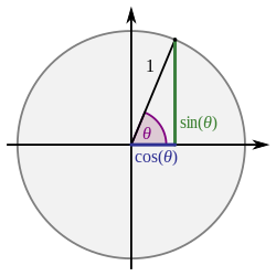


![{\displaystyle [-1,1]}](https://wikimedia.org/api/rest_v1/media/math/render/svg/51e3b7f14a6f70e614728c583409a0b9a8b9de01)


![{\displaystyle (-\infty ,-1]\cup [1,\infty )}](https://wikimedia.org/api/rest_v1/media/math/render/svg/7e3448e2de68557e598967fb8b1f8900260c4a64)


![{\displaystyle \left[-{\tfrac {\pi }{2}},{\tfrac {\pi }{2}}\right]}](https://wikimedia.org/api/rest_v1/media/math/render/svg/c2052f9d4a9c6a14f6db2e4bcd2606bce26d720d)


![{\displaystyle [0,\pi ]}](https://wikimedia.org/api/rest_v1/media/math/render/svg/3e2a912eda6ef1afe46a81b518fe9da64a832751)


![{\displaystyle \mathbb {R} \setminus (-1,1)=(-\infty ,-1]\cup [1,\infty )}](https://wikimedia.org/api/rest_v1/media/math/render/svg/105fc2887189c9dbf0d165542a768dcd97f03069)


![{\displaystyle [\,0,\;\pi \,]\;\;\;\setminus \left\{{\tfrac {\pi }{2}}\right\}}](https://wikimedia.org/api/rest_v1/media/math/render/svg/c913c2c78d11f57ccd118976bfb4b0595e5a2e0e)


![{\displaystyle \left[-{\tfrac {\pi }{2}},{\tfrac {\pi }{2}}\right]\setminus \{0\}}](https://wikimedia.org/api/rest_v1/media/math/render/svg/e84fda7925743a03ffa0aec3fbed76a2967a3012)


![{\displaystyle {\begin{aligned}\sin {\frac {\theta }{2}}&=\pm {\sqrt {\frac {1-\cos \theta }{2}}}\\[3pt]\cos {\frac {\theta }{2}}&=\pm {\sqrt {\frac {1+\cos \theta }{2}}}\\[3pt]\tan {\frac {\theta }{2}}&=\csc \theta -\cot \theta =\pm \,{\sqrt {\frac {1-\cos \theta }{1+\cos \theta }}}={\frac {\sin \theta }{1+\cos \theta }}\\[3pt]&={\frac {1-\cos \theta }{\sin \theta }}={\frac {-1\pm {\sqrt {1+\tan ^{2}\theta }}}{\tan \theta }}={\frac {\tan \theta }{1+\sec {\theta }}}\\[3pt]\cot {\frac {\theta }{2}}&=\csc \theta +\cot \theta =\pm \,{\sqrt {\frac {1+\cos \theta }{1-\cos \theta }}}={\frac {\sin \theta }{1-\cos \theta }}={\frac {1+\cos \theta }{\sin \theta }}\end{aligned}}}](https://wikimedia.org/api/rest_v1/media/math/render/svg/cdc1f00b70f6eddf80b91c17e5f785480bc325a8)
![{\displaystyle {\begin{aligned}\tan {\frac {\eta \pm \theta }{2}}&={\frac {\sin \eta \pm \sin \theta }{\cos \eta +\cos \theta }}\\[3pt]\tan \left({\frac {\theta }{2}}+{\frac {\pi }{4}}\right)&=\sec \theta +\tan \theta \\[3pt]{\sqrt {\frac {1-\sin \theta }{1+\sin \theta }}}&={\frac {\left|1-\tan {\frac {\theta }{2}}\right|}{\left|1+\tan {\frac {\theta }{2}}\right|}}\end{aligned}}}](https://wikimedia.org/api/rest_v1/media/math/render/svg/639270245e163f1afa8682ac8aa12086db43dce1)


![{\displaystyle {\begin{aligned}\prod _{k=1}^{n}\cos \theta _{k}&={\frac {1}{2^{n}}}\sum _{e\in S}\cos(e_{1}\theta _{1}+\cdots +e_{n}\theta _{n})\\[6pt]&{\text{dimana }}S=\{1,-1\}^{n}\end{aligned}}}](https://wikimedia.org/api/rest_v1/media/math/render/svg/219f5560a5a505f3d3c48c68d987097bbb84cb2f)


